The convergence of neural networks
Neural Networks perform well, but how well? Using a statistical framework permits the caluclation of the order of convergence, or to be precise, an upper bound on this order. Some time ago I wrote my Master Thesis on the subject and I decided to post a short summary of some key insights here, lest I might lose track of the basics myself. If you are interested in the whole story, visit my github repo with the whole thesis and code. This post does not have the goal to be as precise as possible, but to convey the general idea behind the calculations. For precise conditions on eg. function spaces or mixing conditions, the reader is referred to the thesis itself.
Considering ANNs as Nonparametric Estimators
To develop asymptotic theory, it is easiest to integrate ANNs into the nonparametric framework. Here, we will focus on the single-hidden-layer ANNs because they are rather easy to manipulate, the results however, generalize to the multilayer case as well.
The parametric form of ANNs
Basic ANNs can easily be written in their parametric form.
\[f(x, \theta) = F\bigg(\beta_0 + \sum_{k=1}^{m}G(\tilde{x}'\gamma_k)\beta_k\bigg),\]where \(m\) is the number of hidden units in the hidden layer.
The Bias Variance Tradeoff
Sieve Estimators
The basic idea of sieve estimation is to use increasingly more complex versions of a base model as more data becomes available. This might sound weird but the rationale behind it is quite simple. Imagine that we want to approximate some unknown function \(f(x)\) on \([a,b]\). With just a few datapoints we might try to approximate the function with an intercept and a slope:
\[f(x) \approx w_0x^0 + w_1x^1,\]where w are some weights. The approximation will be quite rough, but we could add more polynomial terms. We known from Stone-Weierstrass that we can uniformly approximate a continuous function to any desired degree of accuracy with an increasing number of polynomial terms. In the real world, unfortunately, we always have some kind of noise present in the data and just adding more and more terms to a regression equation usually results in strong overfitting. Below is a small graph that shows the approximation properties of a simple linear regression and its polynomial equivalent for polynomial order 2, 5 and 10.
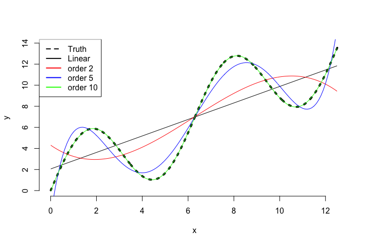
Sieve estimation builds on exactly these two principles. With a suitable base function we will try to approximate a function of interest but keep in mind the bias-variance tradeoff. With more and more data points available, it will become easier to differentiate noise from signal and hence we can allow the equation to contain more terms (and make it therefore more flexible).
To put this into slightly more mathematical terms, we have
\[y_t=\psi_0(x_t) + \varepsilon_t, \quad \mathbb{E}[\varepsilon_t|x_t] = 0,\]for simplicity we assume \(y_t, \varepsilon_t, x_t \in \mathbb{R}\). With the standard least squares approach, the optimal estimator can be written as:
\[\hat{\psi}(\cdot) = \arg\min_{\psi(\cdot) \in \Psi}\frac{1}{n}\sum_{t=1}^{n}(y_t - \psi(x_{t}))^2\]In usual parametric settings, the functional space of \(\Psi\) is limited to a specific form and the parameter vector bound in some (fixed) space \(\mathbb{R}^p\). But, if we assume for example that \(\Psi = =\mathcal{C}^2(\mathbb{R}),\) the space of twice continuously differentiable function on \(\mathbb{R}\), the optimization problem is no longer well posed (as even if we had the possibility of searching over the whole \(\Psi\), there might exists an infinite number of solutions). The sieve approach consists of replacing \(\Psi\) with a series of increasingly complex sieve fuctions that are of a lower dimension. This can be expressed as:
\[\psi \in \Psi_d = \big{\{}f:f(x;\theta)=\sum_{d=1}^{r_n}\theta_d\mathcal{G}_d(x) \big{\}} \quad ,\]where \(d\) is the dimensionality of the sieve and \(\mathcal{G}\) are the so called base functions. There are some conditions on \(\mathcal{G}\) but the one to remember is that the base functions must be dense in the original space. As we saw above, polynomials are dense in the original space (at least in the limit) and as it turns out, already a single hidden layer of an ANN can be too! The use of this is straight forward, by using theoretical approaches derived for other sieve estimators, we can pin down the rate of convergence of neural networks! Because we would have had an infeasible estimation problem we can render the problem into a feasible problem. By acknowledging that in the limit our estimator can approximate any desired function in the specified space but “pretending” to approximate it only in a lower dimesion we can calculate some convergence properties. Our feasible problem then looks somewhat like:
\[\hat{\psi}(\cdot) = \arg \min_{\theta \in \Theta_d}\frac{1}{n}\sum_{t=1}^{n}(y_t - \psi_d(x_t))^2\]In a sense we say that we cannot estimate the “true” \(\psi_0\) but we can estimate a lower dimensional version \(\psi_d\) which, in the limit as \(n \rightarrow \infty \quad \psi_d = \psi_0\). To have well defined properties, we need some conditions of course. For example (and quite obviously) the approximation spaces \(\Theta_d\) must be compact and nondecreasing in \(d\) and \(\Theta_d \subseteq \Theta\). And we must also observe that:
\[\frac{1}{r_n}\rightarrow 0 \quad \text{and} \quad \frac{r_n}{n}\rightarrow 0 \quad \text{as } n \rightarrow \infty\]This ensures that the parameter space is infinite in the limit but that the parameter space increases slower than the sample size. If you are familiar with nonparametric kernel regression these conditions should seem rather familiar. Compared to kernel regression, sieve estimation has the benefit that they are global estimates and not just local approximations (ie. they approximate the function over the whole set of data points).
The order of convergence
For a single hidden layer ANN with ReLU activation functions, the order of convergence can be expressed as:
\[||\hat{\theta}_n - \theta_0|| = \mathcal{O}\bigg{(}[n/\log(n)]^\frac{-(1+\frac{2}{d+1})}{4(1+\frac{1}{1+d})}\bigg{)} ,\]where \(d\) is the input dimension and \(n\) is the sample size.
Some implications
Usually this is the moment when any non-statistician would ask, “so what”?. A tentative answer can be found in the following graphic. Here we compare the above deducted convergence rate to that of a standard nonparametric kernel estimator. It can be expressed as:
\[\mathcal{O} \bigg{(}n^{\frac{-2*\text{order}}{2*\text{order} + \text{dimension}}} \bigg{)}\]If we compare their convergences for specific values (altough this is technically not correct - as we excluded a constant in the big-oh term) we get the following graph:
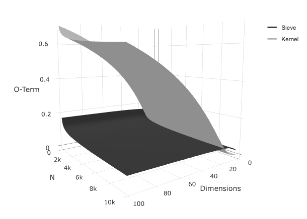
Here we can see the big-oh term given a set of dimension-N (N represents the size of the data). For lower dimensions, the grey surface representing the the big-oh term for the kernel estimator is lower than the dark surface, but only for low values in the dimensions. It seems that the sieve estimators are a lot less sensistive to the curse of dimensionality. Which in turn could help exlplain their popularity in text- and image mining (where dimensions are extremely high). On the other hand, Neural Networks failed spectacularly for low-dimensional time series predictions in, for example, the M4 competition (see eg. the corresponding paper)