Further research
Work on higher orders and subgroups
The last part in this series tries to work on some of the drawbacks that might occure in the simple mechanism that we developed in the post on simulation. Some of it (“the friends-of-friends”) part can already be found in our Article but the work on subgroups goes slightly beyond that.
Higher order connections
We saw in the previous post, that some agents cannot share their whole deductible, as they cannot find “friends” (aka first order connections) that are willing to enter a contract with them or not enough to fill up their desire. This will happen more often if the network becomes more concentrated (which happens in higher-variance cases).
A possibility to overcome this issue is to look further than ones friends. For example, one could try to share some of the residual risk with the friends of his friends. This simply corresponds to the second order connections, that were not already connected to a specific node. Or in set notation:
Given a network \((\mathcal{E},\mathcal{V})\), with degrees \(\boldsymbol{d}\) and some first-level optimization vector \(\boldsymbol{\gamma}_1\), define the subset of vertices who could not share their whole deductible as,
\[\mathcal{V}_{\boldsymbol{\gamma}_1} = \big\lbrace i \in \mathcal{V}: \gamma_i=\sum_{j\in\mathcal{V}}\gamma_{(i,j)} < s \big\rbrace.\]The \(\boldsymbol{\gamma}_1\)-sub-network of friends of friends is \((\mathcal{E}_{\boldsymbol{\gamma}_1}^{(2)},\mathcal{V}_{\boldsymbol{\gamma}_1})\),
\[\mathcal{E}_{\boldsymbol{\gamma}_1}^{(2)} = \big\lbrace(i,j)\in\mathcal{V}_{\boldsymbol{\gamma}_1}\times\mathcal{V}_{\boldsymbol{\gamma}_1}:\exists k\in\mathcal{V}\text{ such that }(i,k)\in\mathcal{E},~(k,j)\in\mathcal{E}\text{ and }i\neq j\big\rbrace\]Now we can assume that everyone would trust the friends of his friends slightly less (or assume they have a slightly different risk profile), so naturally one would share less of the risk with them. In our example we assume that each node wants to share up to \(25\) with a friend but only \(5\) with the friend of a friend. We can see the results below.
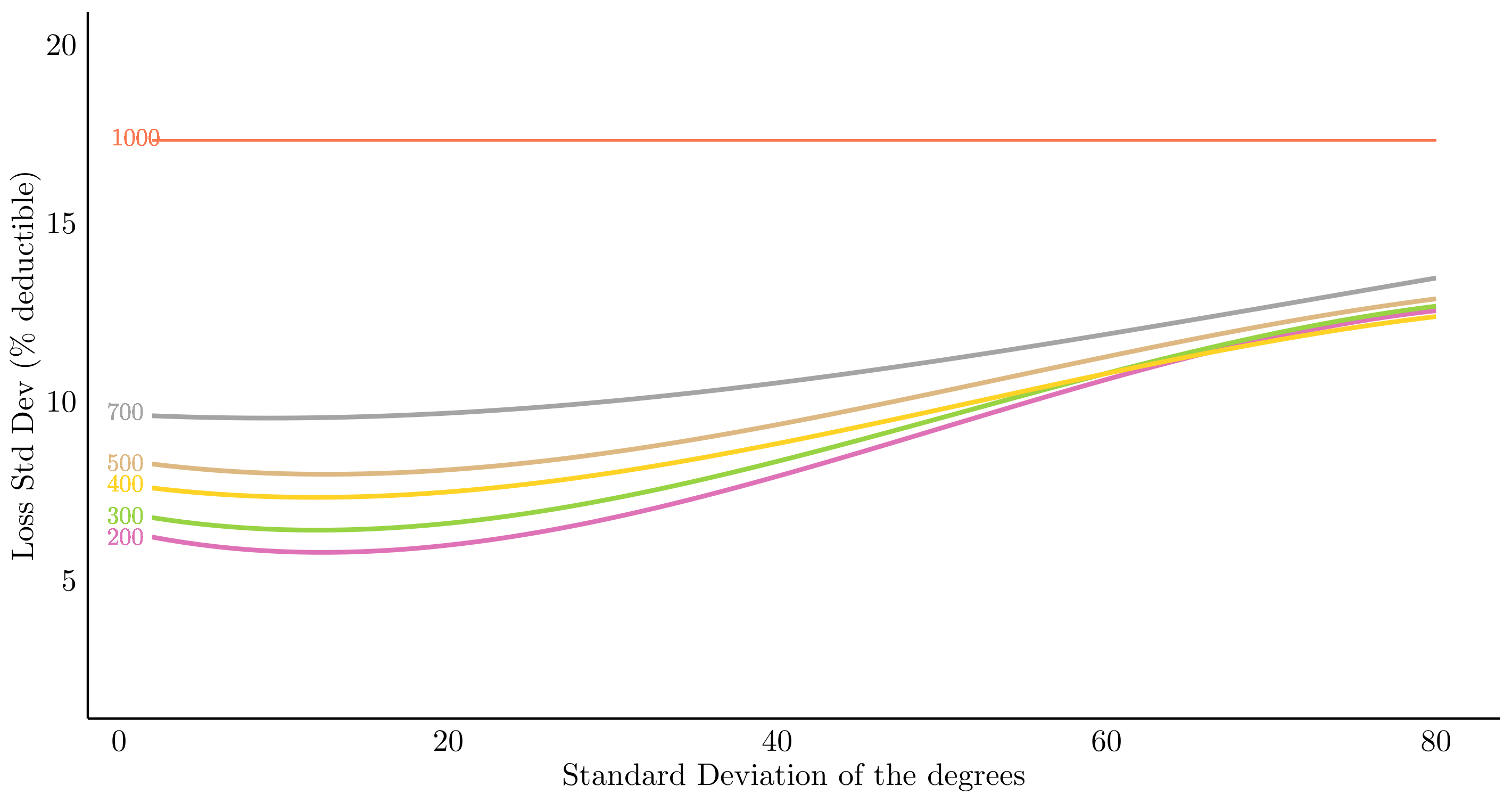
Looks like an improvement already. But under the hood something interesting is going on, best visualized as follows:
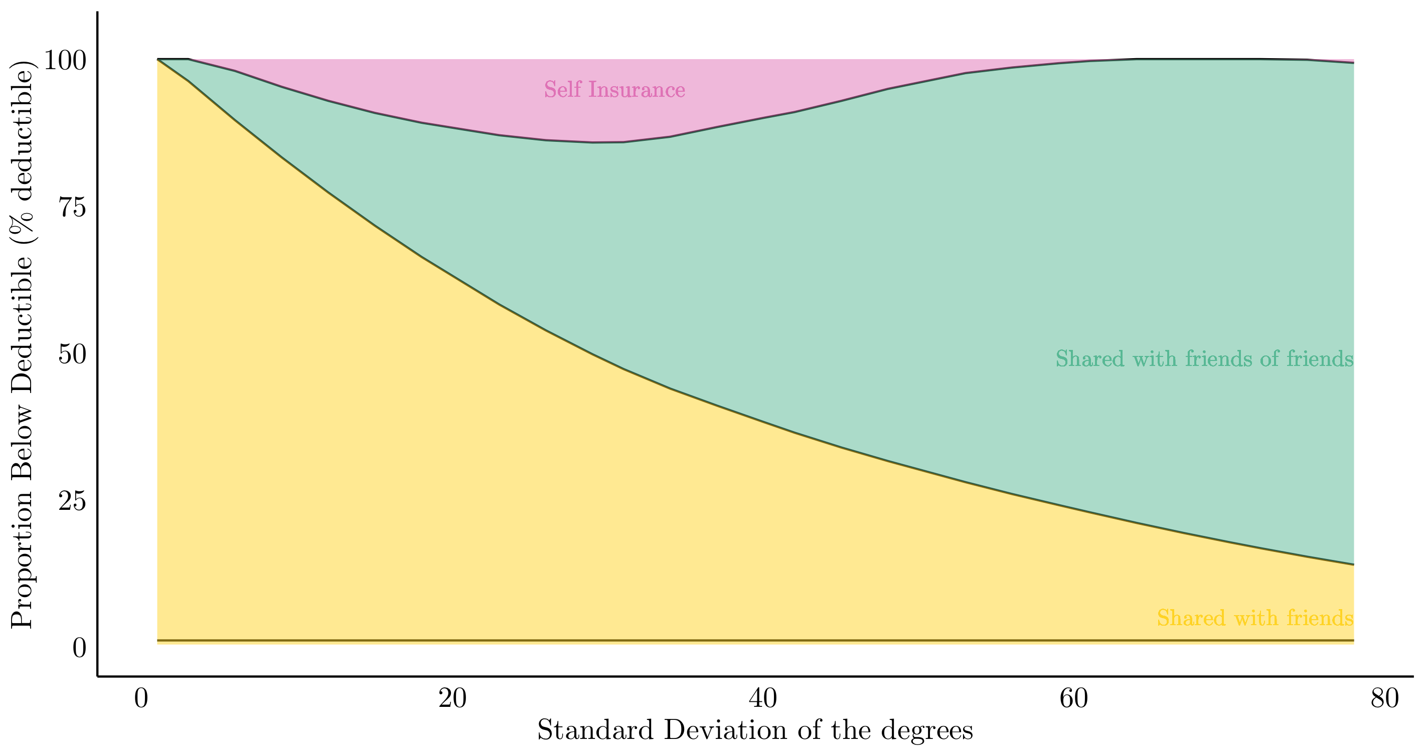
The centralization due to the higher degree variance actually generates “hubs” - really popular agents that help every connected node to have more “friends-of-friends”.
Sparsification of the contracts
In the case of optimal reciprocal engagements, some contributions can be close to zero but not exactly zero, as even a minimal engagement will increase the global optimization problem. In this case it might be beneficial to “shrink” these contributions to effectively zero, especially if those reciprocal contracts have some management fixed costs, without decreasing \(\boldsymbol{\gamma}^*\) too much. This can be achieved by reformulating the linear programming problem into a mixed-integer optimization.
\[\begin{cases} \boldsymbol{z}^\star =\displaystyle{\underset{\boldsymbol{z}\in\mathbb{R}_+^m}{\text{argmax}}\left\lbrace\boldsymbol{1}^\top\boldsymbol{z}\right\rbrace}\\ \text{s.t. }\boldsymbol{T}^\top\boldsymbol{z}\leq s\boldsymbol{1}_m\\ ~~~~z_i \leq My_i,~\forall i\\ ~~~~\displaystyle{\sum_{i}y_i\leq m} \end{cases}\]where \(y_i \in \{0,1\}\) and \(m\) maximum desired non-zero engagements. \(M\) is an upper bound on each \(z_i \in \boldsymbol{z}\) which comes naturally as we look for reciprocal engagements smaller than the specified \(\gamma\). This mechanism will effectively shrink small contributions to zero.
The figure below depicts the trade-off. This mechanism becomes more important for the friends-of-friends problems, where networks with a high degree standard deviation result in second degree adjacency matrices with extremely large \(\lvert\mathcal{E}\rvert\). Intuitively, this allows the global planner to introduce a trade-off between having a large total coverage but a restricted number of contracts.
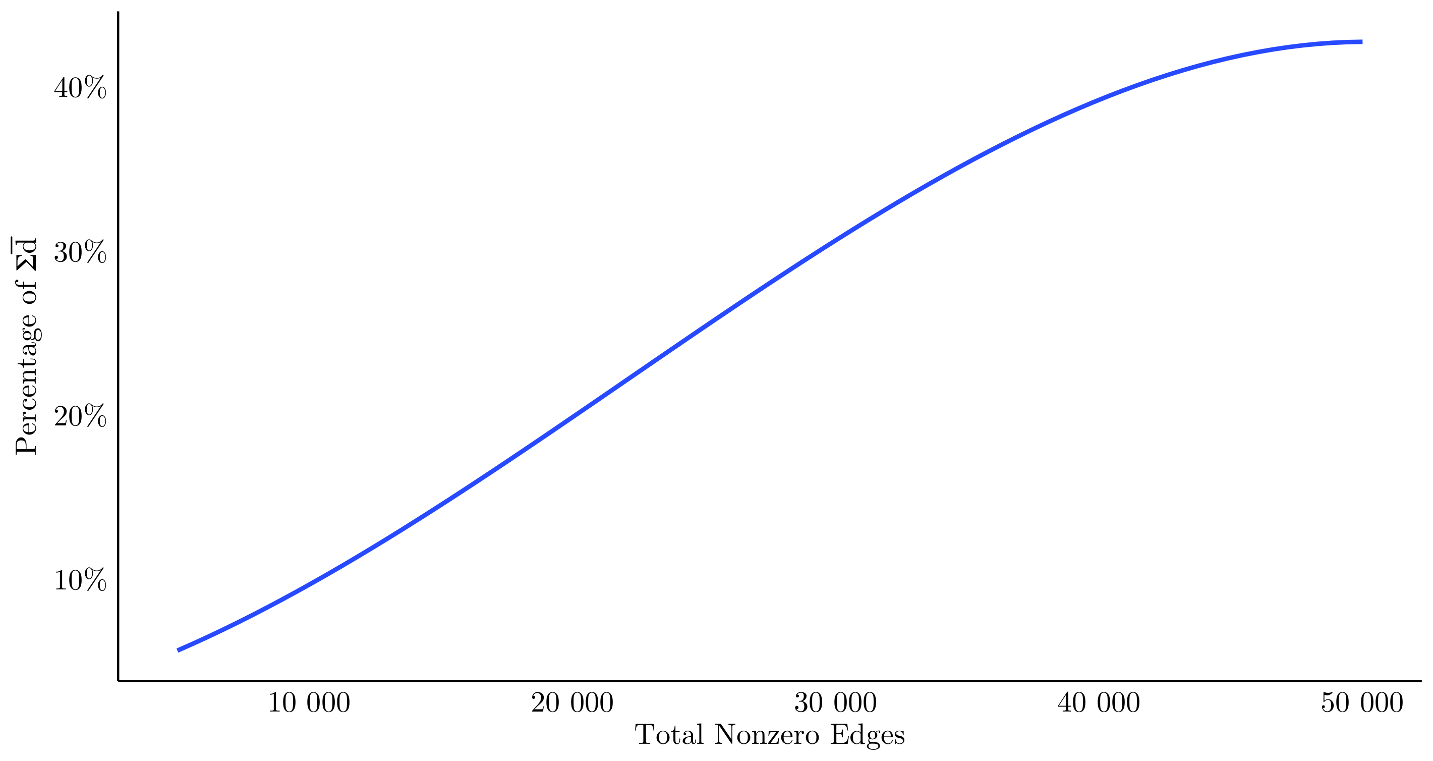
Depicted here is the percentage of the sum of deductibles being shared with different number of non-zero edges. Whereas there is a close to linear trade-off in the middle ground, where a one less edge results in \(-\gamma\) on the total sum, the function plateaus on the right hand side, resulting in a sparser solution with almost the same percentage shared.
Subgroup sharing
Throughout our article, we argued that our assumption of i.i.d. risks is somewhat justified due to homophily which is often encountered in real networks. After all - if people are similar in many aspects of life, they should also be similar in the aspects that make up risk itself.
But even then in those cases there might be some correlation among sub-parts of the network. Imagine an appartement block being on fire - there will be some correlation of the risk, or consider theft insurance which will be correlated based on spatial patterns. An attractive option would be to consider cliques, but we already saw in the post on risk sharing principles that even finding an optimal clique cover is NP-complete. An alternative to finding a clique cover is to find more densly connected subgroups (in the literature often called clustering).
For that we will simulate data based on the lfr-benchmark, as our networks that we generated before do (by construction) not contain an inherit subgraph structure. We then cluster the graph (here using a modularity based approach) and assign to each true subgroup (not the ones retreived by the clustering) a different claim probability and analyse how much risk was shared within the homogenous communities.
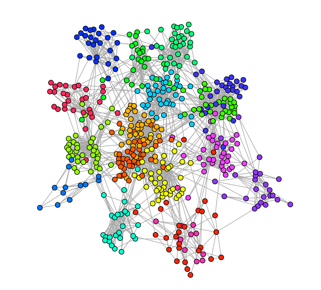
Here we see a smaller clustered subgraph after coloring the clusters with the estimated results.
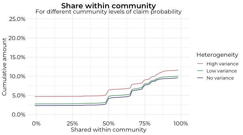
The evaluation in such a setting becomes more challenging, even if we only consider numerical details, there are many nuts and bolts that can be changed (and indeed, will be different in every real world scenario). Here we illustrate how much of the risk is shared within each subgroup. This of course depends on the variance of the Bernoulli parameters across the subgroups and the structure of the networks. In theory, if too much risk is shared with a more risky subgroup, agents have an incentive to deviate, but this should only occur after an initial period. This in turn goes well beyond the scope of our article, but analysing multiperiod dynamics is a natural next step on our endeavour to understand P2P insurance products from a mathematical perspective.