Simulations

In our Article, we run lots of simulations to show that our proposed approach results in better outcomes than the no-insurance case, even for very different types of networks (from regular-poisson-power law degree distributions). Since we work with a deductible of \(s=1000\) the risk sharing scheme will no longer be linear which means we need to simulate the results.

In this blog, you will find a summary of how this was done. For further information check out either the article or the github page.

Basics on the simulations

Since we want to develop a mechanism that holds for a variety of different networks, we need to generate lots of them but still somehow control their underlying nature. Here we assume the simplest form of a network, it is only dependent on the degree distribution vector (this can be simulated with degree.sequence.game with the package igraph).

The idea behind this is easy to explain. We want to derive an insurance mechanism where risk is shared via the edges or a graph \(\mathcal{G}=(\mathcal{V}, \mathcal{E})\). It is well known that if we use i.i.d. risks for every node in the network, the best solution will arise when each node can split its risk with as many other nodes as possible. A starting point for that would be to consider a regular graph (that is - a graph where every node has the same degree \(deg(v_i) = \overline{d}, \quad \forall i \in [ \mathcal{V} ]\)), so if every node shares \(\gamma = \frac{s}{deg(v_i)}\) with every node adjacent to it, we will get the optimal results. But now, consider the images below:

Low degree dist. variance	High degree dist. variance

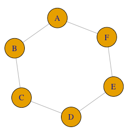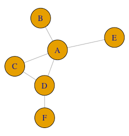Both graphs contain the same number of edges, but the variance of the degree vector obviously changed. Now, it seems a lot more difficult to insure everyone to the same degree in the graph on the right than on the left, for example, nodes B,E,F can only share risk with A or D, and to make matters worse, A has four people to choose from, which means it probably does not want to share risk with all its connections (increasing the chance that B or F might have no insurance at all!).

In larger networks, the same intuition applies. Hence we try to simulate (most) of these simple networks between the regular case (degree vector variance = 0) to very extreme cases (degree vector variance » 0). We opt to do so by the following formula for the degree vector $D$

\begin{equation} D \overset{\mathcal{L}}{=}\min{5+[\Delta],(n-1)}, \end{equation} where \(\Delta\) follows a gamma distribution with mean \(\mu - 5\) and variance \(\sigma^2\). The shift and minimum condition ensures that every node has at least five connections and no multiple edges exist. The advantage of this approach is that by changing the $\sigma$ parameter, degree distributions that resemble a Poisson distribution can be generated just as well as ones that resemble an exponential distribution (ie. models generated by Erdős–Rényi or the preferential attachment method respectively).

For our simulations we generate a graph of \(n=5000\) nodes, with an average degree \(\overline{d}=20\) and let the degree variance vector vary between \(\sigma = [0, 80]\).

A linear program

Now that we have the graph(s), we can pose some possible parameters for the risk facing our \(n\) agents. In our article, we assume that every node is subject to a binary claim probability following some Bernoulli process with \(p=0.1\) (note again, we assume i.i.d. risks across the graph - this is somehow justified by homophily a.k.a. birds of a feather flock together). If a claim occures we add a cost of \(Y_i = 100 + X_i, \quad X_i \sim\Gamma(\frac{900^2}{2000^2}, \frac{900}{2000^2})\) to it. Remember, costs are capped above at \(s=1000\). This setup will result in an expected loss of around \(4.5\%\) of the deductible and a loss standard deviation of around \(17\%\) of the deductible.

Agents can now share their risk by entering contracts with connected nodes. This contract engages them to contribute up to a specified amount in case the other party faces a loss but also receive compensation in case of a loss

Now, the simplest idea is to share risk across all edges in the graph, with some fixed amount for all the contracts (lets say \(\gamma = \frac{s}{\overline{d}}\) as above). This has some suboptimal results though which can be seen blow

Issues on sharing and fairness

Below are two graphs, depicting the results when we propose a simple one-size-fits-all solution as described above. The brown points and corresponding line are what the loss standard deviation for the agents in the network with no insurance. As expected, this value hovers around \(17\%\). In green is the loss standard deviation for the agents under the proposed mechanism. Clearly, the mechanism works quite well (ie. reduces the loss standard deviation for the agents) in networks with low degree variance (which is most often assumed in the previous literature) but it may results in outcomes even worse than the no-insurance case. This is due to the almost star-shaped nature of high degree variance networks. There some nodes possess a hughe amount of connections and loading all of them up with contracts results in (obviously) suboptimal results. We will try to alleviate this issue by issuing optimized contracts for each connection (a variable \(\gamma\) that can effectively be 0)

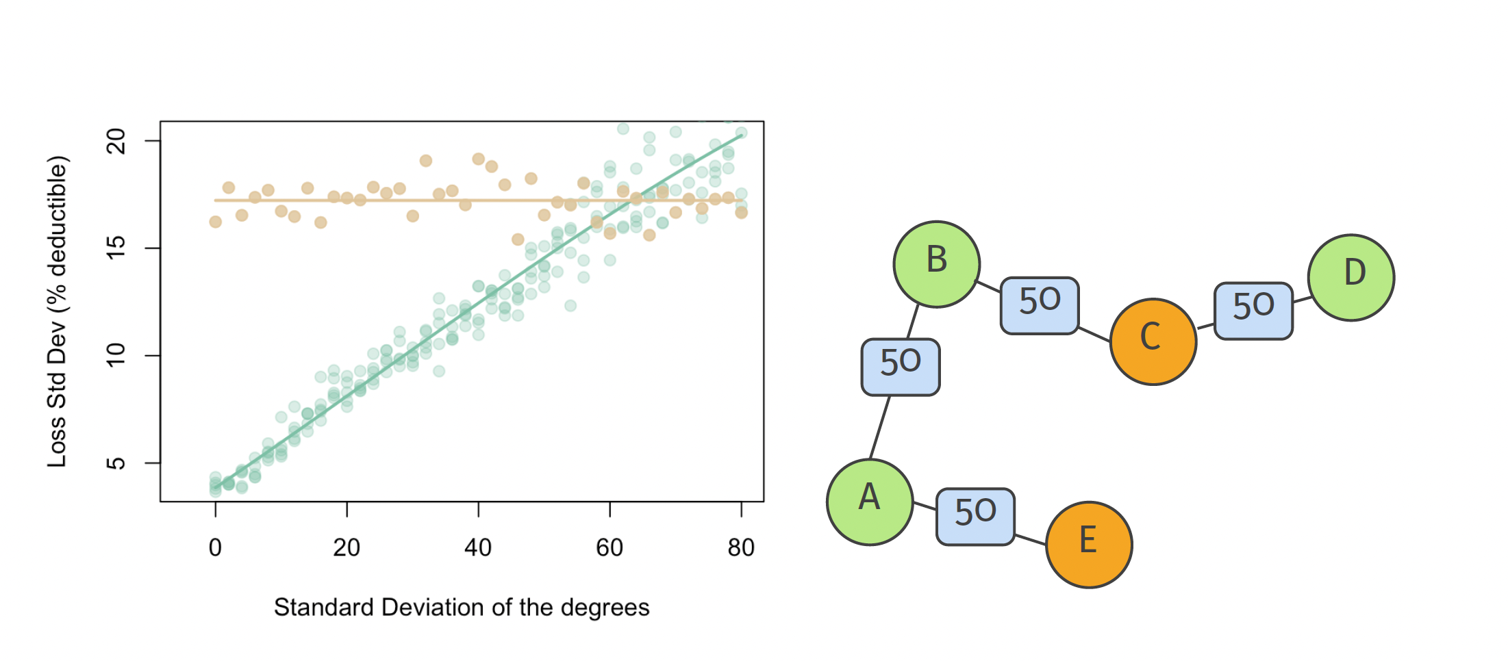
Another issue can be seen on the right. If as much risk as possible is shared with adjacent agents, this might lead to outcomes that are percieved as unfair. Consider the case where nodes C and E have a claim for a total of \(100\) each. For C, the contracts will be activated with B and D and each of them will contribute up to the specified amount (here 50) to C. But then C can cover the entire loss and pays 0, whereas B and D will need to pay altough they did not even have a claim (note that this might be correct ex-ante if they all have the same risk profile but seems rather unfair ex-post). We can mitigate this issue easily tough. Instead of sharing all the risk directly, we can introduce some self-contribution that nodes need to pay first, before and contracts can be activated.

The final mechanism can then be summarised as follows (for a node A):

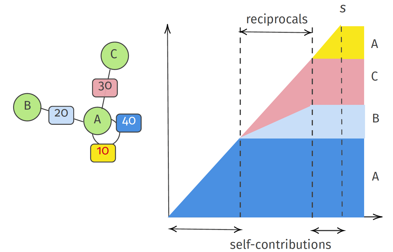
Here node B is willing to share up to \(20\%\) of its risk with A and C up to \(30\%\). The contract also has a specified selfcontribution for \(40\%\). Together this does not cover the entire deductible tough, and A needs to assume the last \(10\%\) again (in case the claim goes above \(90\%\) of the deductible). This last layer can be further optimized later on (see eg. the further research post).

Optimized reciprocal contracts with self-contribution

All of these conditions can be summarised in a linear program:

Thus, formally, we consider the following linear programming problem, where our goal is to maximize the total coverage across our network, but subject to the constraint that every node only wants to assume up to \(s\) units of risk.

where \(s\) is the deductible of the insurance contract and assumed to be the same across all nodes. We then ran 50 simulations for every level of \(\sigma\) between \(0\) and \(80\). The results can be seen below for different amounts of self contributions (1000 means no insurance as the self contribution is equal to the deductible):

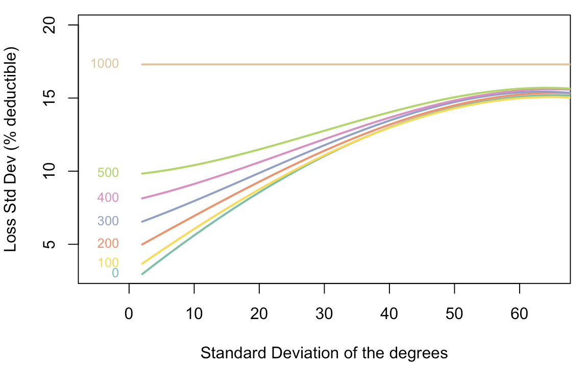
Looks much better right?

There are still some improvements and extensions possible, which we discuss in the further research post