Application
Estimating the Value at Risk
Finally, after considering theoretical stuff in the theory post and finite sample properties in the simulation post we can come to an application. Having been just old enough to start to understand the great recession of 2008, I grew up wondering why so many financial institutions experienced stress in their balance sheets. Later at University, one of my professors mentioned “errors in their VaR” as one of the causes. Instead of only surpassing the VaR around the same amount as predicted, many models underestimated the value at risk by quite a lot.
Besides the numerous disadvantages that the VaR poses (just google it), one possible reason could be model misspecification of the model. Here we give a very simple application of a semiparametric model that could be used instead. We focus on a rather simple model, that we then expand to contain a nonparametric term.
Semiparametric CAViaR
The CAViaR, or Conditional Autoregressive Value at Risk was developed by Engle and Manganelli. It is specified as follows:
\[f_t(\beta) = \beta_0 + \sum_{i=1}^q \beta_i f_{t-i}(\beta) + \sum_{j=1}^r \beta_j l(x_{t-j}),\]where \(f_t\) denotes the estimate of the quantile associated with the VaR. We basically get a autoregressive process of the VaR estimate with a function of lagged covariates. In the spirit of the simulation post we add a nonparametric disturbance term and get the semiparametric form of the VaR:
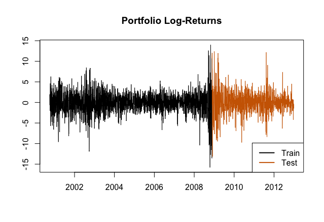
\[f_t(\beta) = \beta_0 + \sum_{i=1}^q \beta_i f_{t-i}(\beta) + \phi(\boldsymbol{x})\]Where the \(\boldsymbol{x}\) vector can contain lagged covariates and the function \(\phi\) will be estimated by the neural network. We then estimate the VaR on both a single stock and a portfolio of stocks and compare their estimates against both the traditional CAViaR model and a GARCH. For the stock the procedure is straightforward, for the portfolios we select among 6 stocks and commodities and construct 50 randomly weighted portfolios and then estimate the VaR. We train the models on a pre-stress period to simulate the same conditions that were available before the great recession and then compare their performance during the stress period. Below a depiction of the train and test sets:

Of course, if we compare predictions, an important indicator is the total number of times that the VaR estimate is exceeded. Since we are dealing with expectations here, we need a test. Luckly there are two test available, the Failures test and the Duration test. If we reject the failure test (p-value smaller than 0.05) that means there is evidence that the model underestimates the VaR. For the duration test we can measure whether there is a temporal correlation between the exceedances, if we reject it, we can further improve the model. We get the following results:
| Garch(2,1) | ANN | Rec-ANN | CAViaR | MGarch(1,1) | M-ANN | CAViaR | |
|---|---|---|---|---|---|---|---|
| Exceedances | 14 | 11 | 12 | 14 | 23.02 | 10.56 | 22.20 |
| Failures Test | 0.23 | 0.75 | 0.54 | 0.23 | 0.52 | 0.02 | 0.50 |
| Duration Test | 0.15 | 0.01 | 0.17 | 0.42 | 0.12 | 0.06 | 0.16 |
| Change \(\int \text{VaR}_\alpha\) | -27.7% | -13.8% | 15.8% | -18.7% | -25.0% | -6.1% | -8.7% |
| Coef. VaR\(_{t-1}\) | 0.66 | 0.82 | 0.46 | 0.55 | |||
| Std. Error | 0.19 | 0.11 |
Where for the portfolios (last three columns), the averages of the tests were calculated. For the exceedances this is just the mean across the portfolios, for the tests it is no longer the p-value (as for the single stock case) but the average rejections of the test (0.50 means the test was rejected 50% of the time). The change in the integrated VaR is a measure of improvement of the model vis-à-vis the unconditional VaR.
Clearly, the parametric models seem less apt to model the VaR of the portfolios. As the “vanilla” ANN approach rejected the duration test, we also modelled the semiparametric ANN-CAViaR with a recursive model, that improved the fit.
Conclusion
To give a very brief conclusion to the series we can add the phrase: much remains to be done. Using previous research, we could extend the convergence bounds for ANNs to include ReLU-Networks, and then studied the properties with finite samples. It seems that ANNs are of better use in higher dimensions. Some evidence from the applications also points into this direction.