Simulations and heuristics
Neural Nets as nonparametric estimators
In the theory post on sieves and of course the Article, we discovered some interesting facts about the rate of convergence of Neural Network type sieve estimators. Namely, whey seem to be less sensitive to the dimensionality of the problem at hand than other well-known nonparametric estimators.
Here you can find the details of some simulations that were run for the article. The goal was to study the properties derived in the theory post but here with only a finite amount of data.
Approximation and Dimensionality
The most important feature that we want to study is how ANN-type estimators behave in different dimensional model settings as compared to other nonparametric estimators. Here they are compared to Kernel type estimators. We begin with a simple case, where there are just two relevant predictors and a noise term, the noise term is assumed to come from a normal distribution. We then successively increase the number of noise terms and number of relevant predictors. In short, the setup looks as follows:
The high dimensional model 1 is generated according to the process: \begin{equation}\label{apB:high_dim_1} y_i = \sum_{i=1}^{k}f_i(X_i) + \varepsilon_i \end{equation}
\[k={2,5,10,15}, \;\;\; X_i= \begin{cases} \sim \textnormal{Unif}([0,3]), & \text{relevant} \\ \sim \textnormal{Unif}([-1,1]), & \text{otherwise} \end{cases}, \;\;\; \varepsilon_i \sim \mathcal{N}(0, 9^2)\]To get a variety of different functions that might be hard to approximate using a parametric model, they take the rather funky forms as defined in the table below.
| function | definition |
|---|---|
| \(f_1\) | \(3.5\sin(x)\) |
| \(f_2\) | \(8\log (\max(\mid x\mid,1) )\) |
| \(f_3\) | \(2x^4\) |
| \(f_4\) | \(-0.4(x^2 + x^3 + 0.1\log(\max(\mid x \mid,0.5)))\) |
| \(f_5\) | \(-4x^3\) |
| \(f_6\) | \(7x^2\) |
| \(f_7\) | \(2\log(\max(\mid x\mid, 0.3))^3\) |
| \(f_8\) | \(\mid x \mid\) |
| \(f_9\) | \(-(0.9x^2 + x^3)/(\max(\sin(x)+2x^5,0.9))\) |
| \(f_{10}\) | \(-4\cos(x)\) |
| \(f_{n > 10}\) | \(x\) |
The functions generating the high dimensional model. If the number of relevant predictors exceeds 10, the functions the subsequent predictors are just linear additive terms. Note that all generated models contain the number of nuisance parameters indicated in addition to the gaussian error term.
That much for the setup, now to the results:
| Relevant predictors | ||||
|---|---|---|---|---|
| Noise Terms | 2 | 5 | 15 | |
| 1 | 6.11\(^*\) | 18.31\(^*\) | 59.13 | |
| Local Linear (Kernel) | 10 | 28.98 | 46.48 | 79.30 |
| 20 | 44.02 | 66.65 | 97.99 | |
| 1 | 22.33 | 33.99 | 41.86\(^*\) | |
| ANN | 10 | 27.10\(^*\) | 36.85\(^*\) | 47.03\(^*\) |
| 20 | 34.87\(^*\) | 43.27\(^*\) | 51.72\(^*\) |
Here we see the results from 50 simulations each, when we consider the RMSE on a test set. The \(^*\) denotes the lowest RMSE across the two different models.
Inference of Semiparametric models
Another interesting part when working with Neural Networks is how they behave if we mix them with a standard parametric model. From an application side, eg Zhang proposed a mix of an ARIMA model with a ANN and found that they perform better as either model in isolation. Further, in the M4 Competition which was analysed by Spyros Makridakis and colleagues found that mixing traditional estimators and machine learning models also resulted in the best forecasts throughout the competition. So instead of focusing on the predictive performance, we conduct a simulation that tries to estimate a linear parameter while having nonlinear disturbances that can be estimated with a neural network.
For that we set up a problem that can weight up the benefits of ANNs as compared to parametric models. Consider the following functions, which is closely related to the experiments of Gao and Tong
\[y_t = \beta_1 v_{t-1} - \beta_2 v_{t-2} + \Big(\frac{x_{t-1} + x_{t-2}}{1 + x_{t-1}^2 + x_{t-2}^2}\Big)^2 + \varepsilon_t, \quad t=1,...,1250\] \[\beta_1 = 0.47, \beta_2=-0.45\] \[v_t = 0.55v_{t-1} - 0.42v_{t-1} + \delta_t, \quad x_t = 0.8\sin(2 \pi x_{t-1}) - 0.2\cos(2 \pi x_{t-2}) + \eta_t\] \[\varepsilon_t \sim \mathcal{N}(0,0.5^2), \quad \delta_t,\eta_t \sim \text{Unif}[-0.5,0.5]\]We then compare the following:
- A parametric model that is specified to the true functional form (usually unknown to the researcher, but should yield the best results
- A parametric model that will have the nonlinear part misspecified
- A fully nonparametric ANN
- A “hybrid” semiparametric ANN that contains both linear terms and a nonparametric correction term
- A semiparametric model where the nonlinear term is estimated by a kernel density estimator
Note, that we are in the low dimensional case here, so we would expect the kernel based model to perform better than the ANN. We compare both the RMSE and this time around also the integrated squared bias and variance for the semiparametric estimators:
| Model | RMSE | \(\int \text{Bias}^2\) | \(\int \text{Var}_e\) |
|---|---|---|---|
| True | 0.4944 | ||
| Linear | 0.5199 | ||
| ANN | 0.5495 | ||
| Semi-ANN | 0.5061 | 0.0012 | 0.0072 |
| Semi-Kernel | 0.0012 | 0.0061 |
Again for each model 50 simulations were carried out. Clearly, the true model beats any other estimation - but more interestingly the semiparametric specification using a neural network performed better than the fully nonparametric specification of the neural network. Inference wise, it is still outperformed by the Kernel based semiparametric model though.
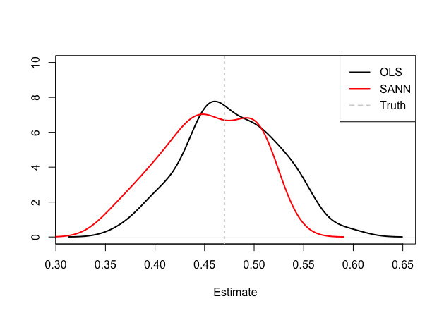
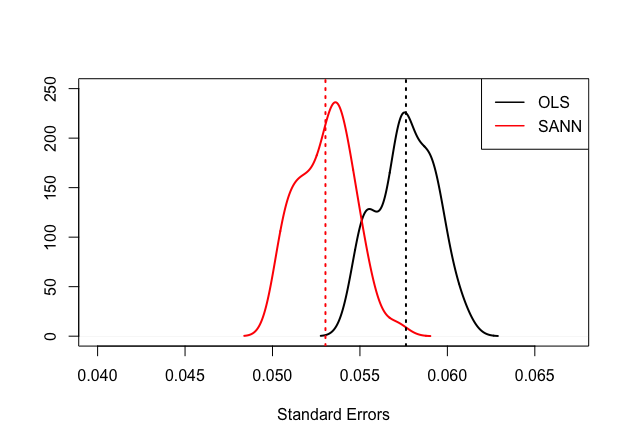
The linear model should still provide unbiased estimates, but they should be less efficient than the same parameters estimated by the semiparametric ANN, as can be seen in the figures below:


So even if a fully nonparametric estimator is available, it might be worth considering a semiparametric approach, not only because it seems to work better in practice, but also because we can infer properties of our model parameters.